rts: an R package for raster time series analysis
‘rts’ is an R package, aims to provide classes and methods for manipulating and processing of raster time series data. There is already a very nice package for handling and analyzing raster data (i.e. package: raster). Several packages have also been developed for handling time series data (e.g. xts package). ‘rts’ simply puts some capabilities from the ‘raster’ and ‘xts’ packages together to provide new classes of raster time series data as well as a framework for analyzing this type of data.
At the current stage, the package has provided the classes and some basic functions, but it is under development and will be extended by adding numerical routines for some specific analysis.
This article aims to demonstrate how this package can be used given some simple examples:
Creating a raster time series object
Two classes, namely ‘RasterStackTS’ and ‘RasterBrickTS’, are introduced by ‘rts’ package for handling raster time series data. These classes have RasterStack or RasterBrick (introduced by package ‘raster’), and xts (introduced by package ‘xts’) classes inside. To create either of these classes, you should have a series of raster files (e.g. satellite images) and the date/time information corresponding to these rasters. Here is an example, we have 4 raster files in the format of grid ascii,
library(rts)
# location of files
path <- system.file("external", package="rts")
# list of raster files:
lst <- list.files(path=path,pattern='.asc$',full.names=TRUE)
lst
# creating a RasterStack object
r <- stack(lst)
d <- c("2000-02-01","2000-03-01","2000-04-01","2000-05-01") # corresponding dates to 4 rasters
d <- as.Date(d)
# creating a RasterStackTS object:
rt <- rts(r,d)
# or alternatively you can simply use the list of files as the first argument:
rt <- rts(lst,d)
rt

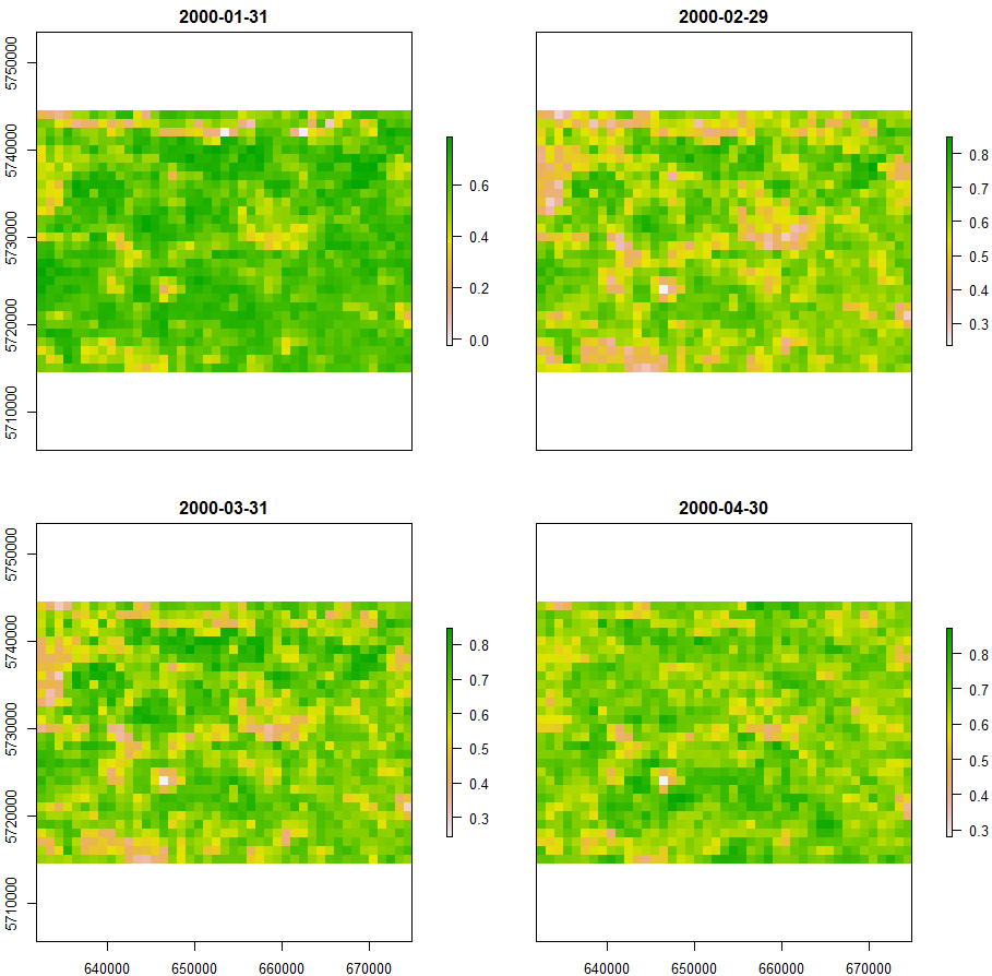
You can use plot function to plot raster layers inside the object:
plot(rt)

Reading and writing raster time series
A raster time series object can be phisically written in working directory using write.rts function. The function creates a folder in the working directory in which a raster brick object is created followed by a text file in which the relevant date-time information is stored. read.rts function can also be used for reading an rts object. Following you will see how the rt object (from previous section) can be written and read using the mentioned functions:
write.rts(rt,"rtfile") # writing n into the working directory
rt <- read.rts("rtfile") # reading nf from the working directory
rt
Apply a function over specified time intervals
Using period.apply function, a specified function can be applied at each cell (pixel) over specified time period. The date/time period can be defined in INDEX argument by introducing a numeric vector in which each number specifies the end point of a date/time period. For example, c(10,20,30) introduces three periods of date/time, first starts from the first raster and ends to the 10th raster in a raster time series object, and the second period starts from 11th raster and ends to 20th raster and so on. If there is more than 30 rasters inside the raster time series object, a 4th period will be included to the selected period which starts from 31st raster and ends to the last raster in the raster time series object.
There is a function, named endpoints, can be used to extract endpoints of the date/time periods based on a date/time base (e.g. seconds, minutes, hours, months, quadrants, years).
A function can be specified in FUN argument. This function should return a single value and is applied at each cell over the specified date/time period. Therefore, a raster will be calculated for each period and the end of the date/time period will be assigned to it in the output raster time series object.
Following you will see an example, a raster time series object including 113 NDVI indices with monthly periodicity from 2000-02-01 01 to 2009-12-01 has been read and several examples show how period.apply can be used:
file <- system.file("external/ndvi", package="rts")
ndvi <- rts(file) # read the ndvi time series from the specified file ndvi
ep <- endpoints(ndvi,'years') # extract the end index on each year period
ndvi.y <- period.apply(ndvi,ep,mean) # apply the mean function on each year ndvi.y
#---------
ep <- endpoints(ndvi,'quarters') # extract the end index on each quarter of a year
# a function:
f <- function(x) {
if (min(x) > 0.5)
mean(x) else 0
}
ndvi.q <- period.apply(ndvi,ep,f) # apply the function f on each quarter
